fred <- function(id) {
  d <- read.csv(paste0("https://fred.stlouisfed.org/graph/fredgraph.csv?id=", id))
  d <- data.frame(date = as.Date(d[[1]]), value = suppressWarnings(as.numeric(d[[2]])))
  d[!is.na(d$value), ]
}

ecb <- function(key) {
  d <- read.csv(paste0("https://data-api.ecb.europa.eu/service/data/", key, "?format=csvdata"))
  t <- d$TIME_PERIOD
  t <- ifelse(nchar(t) == 7, paste0(t, "-01"), t)   # monthly "YYYY-MM" -> date
  data.frame(date = as.Date(t), value = d$OBS_VALUE)
}

# Country averages of OECD immediate (interbank) rates since 2000
cc <- c("US", "GB", "JP", "CA", "CH", "AU", "NZ", "SE",
        "NO", "DK", "KR", "MX", "PL", "HU", "CZ", "ZA")
rates <- do.call(rbind, lapply(cc, function(iso) {
  d <- fred(paste0("IRSTCI01", iso, "M156N"))
  d <- d[d$date >= as.Date("2000-01-01"), ]
  data.frame(iso2 = iso, mean = mean(d$value), sd = sd(d$value))
}))

dfr <- ecb("FM/D.U2.EUR.4F.KR.DFR.LEV")   # ECB deposit facility rate, daily

brk <- data.frame(
  date  = as.Date(c("2008-10-15", "2014-06-11", "2022-07-27")),
  label = c("Financial crisis", "Negative rates", "Hiking cycle")
)

ff  <- fred("FEDFUNDS")
ff  <- ff[ff$date >= as.Date("2000-01-01"), ]
ext <- ff[c(which.min(ff$date), which.max(ff$value), which.min(ff$value),  which.max(ff$date)), ]

m3 <- ecb("BSI/M.U2.Y.V.M30.X.1.U2.2300.Z01.E")   # euro area M3, EUR millions
Monetary Policy Visualization
Financialization and Household Debt
Patrick Mokre
November 16, 2026
Central Banks, Banks, Firms and Households
Conventional Central Bank Policy
Interest rates
Central banks mostly target interest rates through [very short-time] credit (overnight).
The target is a range of auction results.
Lower interest rates should cheapen investment, consumption, exports.
Exchange rates
Appreciating a currency makes imports cheaper and exports more expensive.
Exchange rates are targeted through supply-demand pricing, by releasing or buying up own currency.
However, interest rate interventions also change the exchange rate, lower interest decreases demand for domestic assets and thereby domestic currency.
Multiplicators of Central Bank Policy
Actual firm and consumer decisions are not very sensitive to short-term interest rates. Much investment is self-financed, consumption requires saved down payments.
Central bank policy can however be effective through multipliers, that is, someone else amplifying the effects.
Bank Lending Channel
Banks are the main financing channel for firms that cannot afford to issue stock or bonds. Banks’ decisions not to loan money are often the end of story.
Central banks changing the lending environment leads to firms receiving funds that would otherwise have received zero funds (not more expensive loans).
Open market operation: central bank buys securities from commercial bank, commercial bank earns less income on securities, has to lend more for revenue.
Higher level interventions include changing regulation to make sure banks can continue loaning during financial contraction.
Balance Sheet Channel (Credit Worthiness)
Monetary policy can also change the (apparent) credit-worthiness of households, increasing the credit available to them, and thereby consumer demand.
Expansionary policy increases (inflates) asset values, which can be leveraged in loans.
Lower interest rates decrease repayment burden, increasing profits, firm valuations and firm-related assets.
Asset Price Channel
A fall in the interest rate increases (inflates) prices of stock and real estate.
Fundamental stock prices are assumed to be the present value of future income minus credit cost, the latter factor decreases.
On top of that, expectations of resale prices drive stock prices, which also increase when credit cost falls.
Borderline investment projects become profitable when credit cost decreases, increasing investment for these operations.
Financial Crisis
In financial crisis, increased bankruptcies and opaque network effects decreases confidence in repayment, almost shutting off credit.
This shut off the traditional policy channel for central bank policy.
Unconventional monetary policy included zero lower bound policies, but also strategic purchases of toxic assets.
Financialization
Stockhammer 2010
Financialization (in the economic sense): post-Fordist move towards credit- rather than income-fueled demand regimes after the shareholder revolution.
Often, growth rates react positively on aggregate demand.
Demand can be debt-financed if financial institutions and regulations allow for it: credit availability, credit worthiness and credit affordability.
Banking norms, shadow banking, faster financial markets and liberalization decreased cost of and barriers to credit.
Creates two growth model: export-oriented and credit-financed.
Firms
For firms, increased access to financing comes with increased exposure to financial markets: shareholder interests.
Shareholder interest is furthered by asset price inflation, prioritizing “downsize and distribute” over “retain and reinvest”.
Extreme case: Debt-financed stock buyback programs to increase stock value.
Consequences: Crowd-out of investment and wages, studies suggest causal link.
Households
For households, debt-financed consumption subsidizes income. (Housing) asset price inflation increase credit worthiness.
Households increase borrowing, mainly mortgages, but also consumer credit and even payday loans.
Allows for increase of consumption standards under stagnating incomes.
Increases effective demand without increasing wage cost.
Financial sector
Financializtaion challenges conventional central banking, creates more frequent obstructions of the policy channel.
Increased importance of the less-regulated shadow bank sector.
Key role as lender of last resort.
Manage structural deficiencies (wage suppression and demand deficiencies) through consumer credit.
Stabilize an increasingly unstable (financial instability hypothesis) and under-regulated (financial liberalization) economy.
Plotting
geom_label_repel
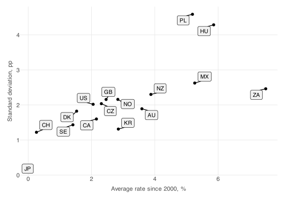
Labels in a scatterplot
geom_density
ggplot(rates, aes(mean, sd)) +
  geom_point(size = 1.5) +
  geom_label_repel(aes(label = iso2), size = 3, fill = "grey95",
                   min.segment.length = 0, seed = 1) +
  labs(x = "Average rate since 2000, %", y = "Standard deviation, pp") +
  theme_void() +
  theme(axis.text        = element_text(colour = "grey30", size = 9),
        axis.title.x     = element_text(colour = "grey30", size = 9, margin = margin(t = 6)),
        axis.title.y     = element_text(colour = "grey30", size = 9, angle = 90, margin = margin(r = 6)),
        panel.grid.major = element_line(colour = "grey90", linewidth = 0.3),
        plot.margin      = margin(10, 10, 10, 10))
annotate(“label”)
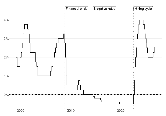
Label annotations
annotate(“label”)
ggplot(dfr, aes(date, value)) +
  geom_vline(xintercept = brk$date, linetype = "dotted", colour = "grey50") +
  geom_hline(yintercept=0, color="black", linetype="dashed") +
  geom_step() +
  annotate("label", x = brk$date, y = 4.6, label = brk$label,
           hjust = 0, size = 3, fill = "white") +
  scale_y_continuous(labels = label_percent(scale = 1)) +
  theme_void() +
  theme(axis.text          = element_text(colour = "grey30", size = 9),
        panel.grid.major.y = element_line(colour = "grey90", linewidth = 0.3),
        plot.margin        = margin(10, 10, 10, 10))
Axis labels
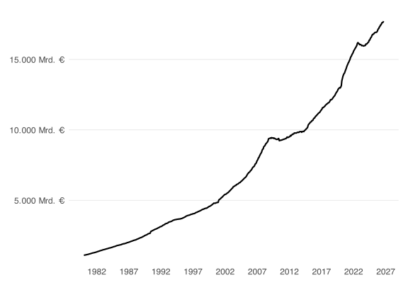
Axis labels
Axis labels
ggplot(m3, aes(date, value)) +
  geom_line(linewidth=0.75) +
  scale_y_continuous(
    labels = label_currency(prefix = "", suffix = " Mrd. €", scale = 1e-3,
                                  big.mark = ".", decimal.mark = ",")
  ) +
  scale_x_date(date_breaks = "5 years", date_labels = "%Y") +
  theme_void() +
  theme(axis.text          = element_text(colour = "grey30", size = 9),
        axis.text.y        = element_text(hjust = 1, margin = margin(r = 4)),
        panel.grid.major.y = element_line(colour = "grey90", linewidth = 0.3),
        plot.margin        = margin(10, 10, 10, 10))
Labels replacing axis labels
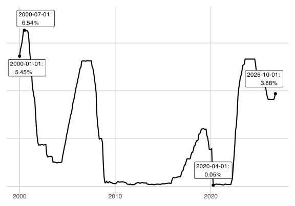
Info Labels instead of axis labels
Labels replacing axis labels
ggplot(ff, aes(date, value)) +
  geom_line(linewidth=.75) +
  geom_point(data = ext) +
  geom_label(data = ext, aes(label = paste0(date, ": \n", sprintf("%.2f%%", value))),
             vjust = c(1.2, -.2, -.4, -.4), hjust=c(.3, .2, .5, .8), size = 3, fill="white") +
  scale_y_continuous(expand = expansion(mult = c(0.05, 0.15))) +
  theme_void() +
  theme(axis.text.x = element_text(colour = "grey30", size = 9),
        plot.margin = margin(10, 10, 10, 10)) +
  theme(panel.grid.major=element_line(color="grey", linewidth=.3),
        plot.margin        = margin(10, 10, 10, 10))
PI 0588 Economic Policy (Applied track) | Winter term 2026